On our last task in the ECNA, we struggled quite a bit, trying to do stuff with convexity and optimization. In the last half hour of the contest, I noticed it could be reduced to the Hungarian Algorithm but did not know how to implement it, so I passed it to my (super smart) teammate to code. According to him, it was something he learned a long time ago and immediately forgot, relying on the prewritten code in kactl instead. So I figured I should do the same thing---learn it and forget it. The first part entails learning it, though, so I've compiled the key parts of the algorithm here.

Problem: There is a fixed $n\times n$ matrix given. You select $n$ numbers in the grid with exactly one from each row and column. Determine the minimum possible sum of the selected numbers.

For example, with

$$M = \begin{bmatrix} 1&4&3\\ 2&11&12 \\ 5&13&14 \end{bmatrix} \quad\implies\quad \begin{bmatrix} 1&4&\boxed{3}\\ \boxed{2}&11&12 \\ 5&\boxed{13}&14 \end{bmatrix},$$

selecting the $2$, $13$, and $3$ gives the minimal possible sum $2+13+3=18$. Evidently, being greedy doesn't work---if we were to start off by choosing the lowest number, $1$, our final sum would be $26$, which is suboptimal.

A brute force solution must look through $n!$ possible selections, which is much too slow. Instead, the Hungarian Algorithm solves this problem in $O(n^3)$, and runs even faster in practice.

Algorithm: Observe that if the same number $-c$ is subtracted from an entire row (or column), every selection will experience the same $-c$, and thus relative to each other, the optimal selection will not change. This essentially gives us $2n$ degrees of freedom to manipulate the matrix.

Our goal is to get the matrix into the following form:

• All entries are nonnegative, and
• There is a selection with all $0$s

At this point, the selection of $0$s is clearly optimal, so the answer to the problem would then just be the sum of the corresponding numbers in the original matrix.

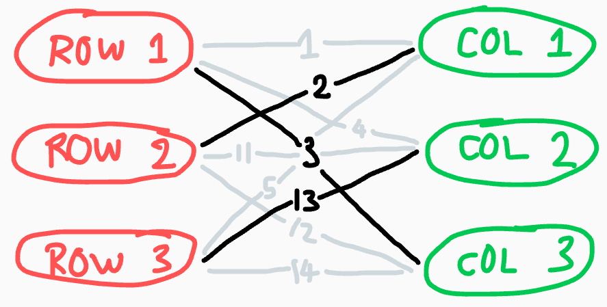
The main part of the algorithm reads more naturally if we first transform the matrix into a bipartite graph. Specifically, suppose we have $n$ vertices representing the rows, and $n$ vertices on the other side representing the columns, and every cell in the grid corresponds to an edge between a row vertex and a column vertex. The above example would become

Then subtracting $-c$ from a row/column is equivalent to assigning a potential $p_i = c$ to a vertex. But, in order to keep all the entries nonnegative, we have the constraints $p_x + p_y \leqslant M_{xy}$ for each edge of the bipartite graph.

Further, whenever $p_x + p_y = M_{xy}$, we will call the edge $xy$ tight, as we are no longer allowed to increase $p_i$ or $p_j$ without decreasing the other under the constraints. These tight edges are equivalent to an entry of the matrix being $0$, so our goal of finding a selection of $0$s in the matrix translates into finding a perfect matching of tight edges in the graph.

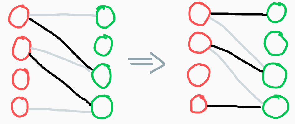
The algorithm seeks to build up a matching on tight edges starting from scratch (zero edges). Our main technique to improve the matching involves finding an augmenting path (shown below). These consist of alternating unmatched and matched tight edges, which allow us to relabel the matching with an extra edge:

To find an augmenting path, start a depth-first-search from any unmatched red vertex. For each red vertex encountered, traverse its tight edges to green vertices---if any of them are unmatched, then we have an augmenting path. Otherwise, from those green vertices, follow the edges in the matching up to new red vertices again, and repeat.

However, at some points of the algorithm (such as the very beginning), the current potentials have not created enough tight edges to find an augmenting path. In this case, the DFS ends with all leaves being red.

Here, we seek to induce more tight edges. Suppose we add $+c$ to each visited red vertex and subtract $-c$ from each visited green vertex.

• Any edge between an unvisited red vertex and an unvisited green vertex is untouched,
• Any edge between a visited red vertex and visited green vertex has the same sum of potentials as before,
• Any edge between an unvisted red vertex and a visited green vertex lowers its sum of potentials by $-c$, hence still satisfies the constraints, and
• Any edge between a visited red vertex and an unvisited green vertex increases its sum of potentials by $+c$. But since the DFS has ended, none of these edges are currently tight.

So if we pick $c$ as the minimum slack $M_{xy}-p_x-p_y$ over all the edges in the last category, we induce another tight edge there. On the other hand, this new edge allows us to continue the DFS to a new vertex. Since there are only $n$ vertices, after $n$ iterations of this subroutine, we are guaranteed to find an augmenting path.

The algorithm is roughly as follows:

for _ in range(n): #extend the matching n times
	start a DFS from an unmatched row vertex
	while (no augmenting path):
		compute minimum slack
		update potentials
		continue the DFS
		

The while loop runs at most $n$ times per extension, so at most $n^2$ times total. Inside, updating potentials takes $O(n)$ time, but naively computing minimum slack over the edges in the 4th category takes $O(n^2)$ time, so the current complexity is $O(n^4)$.

This can be optimized as follows: Suppose we have an array, that for each green (column) vertex, stores the minimum slack to any visited red vertex.

• When we go to compute the minimum slack in the inner loop, the answer is just the minimum of the values of the unvisited vertices in the array, which can be found via a simple $O(n)$ pass.
• When we update potentials, every slack simply decreases by $-c$, so we can update the array in $O(n)$ time.
• When a new red vertex is visited, we can look through its edges and update each slack of the array if the new slack is smaller, also in $O(n)$ time.
  (This is the biggest timesave, as we only look at the slack of each edge once per DFS as opposed to on every iteration of the inner loop).

Therefore, this optimization reduces the time complexity to $O(n^3)$. At the same time, each DFS may find an augmenting path before we have to make $n$ potential updates, so the practical runtime is somewhat faster (i.e. $n=1000$ could still work in $<5$ seconds).